Introduction to Neural Networks
Image kernel convolution
The iris example worked well but the big downside is that it required manual processing of the real-world data before it could be modelled. Someone had to go with a ruler and measure the lengths and widths of each of the flowers. A more common and easily obtainable corpus is images.
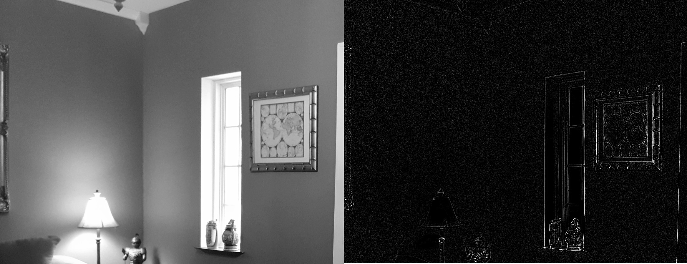
There have been many advancements in image analysis but at the core of most of them is kernel convolution. This starts by treating the image as a grid of numbers, where each number represents the brightness of the pixel
$$ \begin{matrix} 105 & 102 & 100 & 97 & 96 & \dots \\ 103 & 99 & 103 & 101 & 102 & \dots \\ 101 & 98 & 104 & 102 & 100 & \dots \\ 99 & 101 & 106 & 104 & 99 & \dots \\ 104 & 104 & 104 & 100 & 98 & \dots \\ \vdots & \vdots & \vdots & \vdots & \vdots & \ddots \end{matrix} $$Define a kernel
You can then create a kernel which defines a filter to be applied to the image:
$$ Kernel = \begin{bmatrix} 0 & -1 & 0 \\ -1 & 5 & -1 \\ 0 & -1 & 0 \end{bmatrix} $$Depending on the values in the kernel, different filtering operations will be performed. The most common are:
- sharpen (shown above)
- blur
- edge detection (directional or isotropic)
The values of the kernels are created by mathematical analysis and are generally fixed. You can see some examples on the Wikipedia page on kernels.
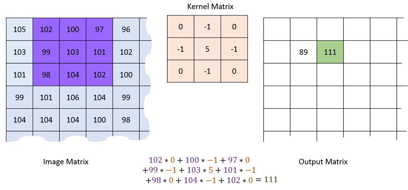
Applying a kernel
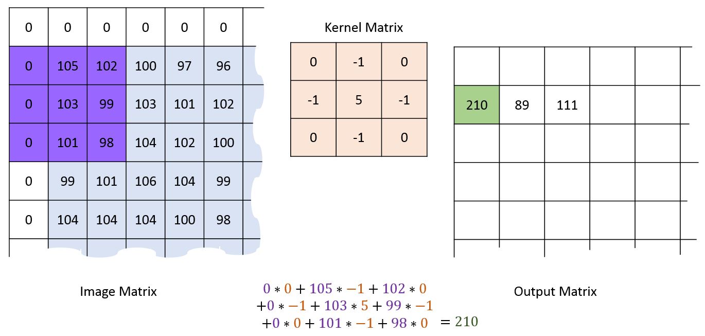
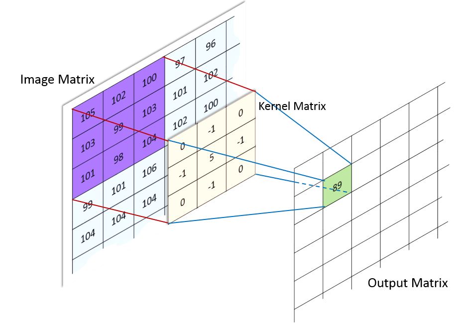
This kernel is then overlaid over each set of pixels in the image, corresponding values are multiplied and then the total is summed:
First pixel
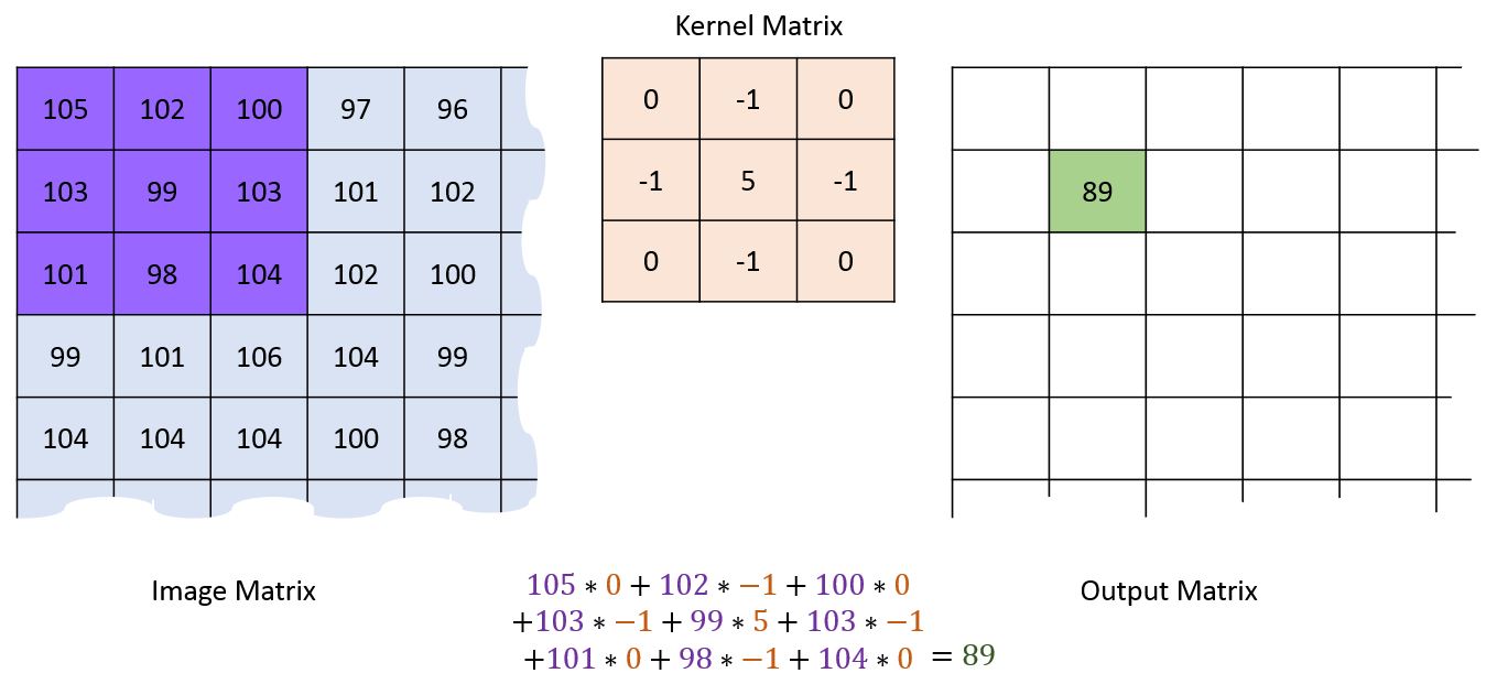
Second pixel
Dealing with edges